THE IMPROVED ARTEMIS–Jean
Louis Steinberg (ARTEMIS-IV) MULTICHANNEL SOLAR RADIO SPECTROGRAPH
OF THE
UNIVERSITY OF ATHENS
Abstract. We present the lately (2002) improved solar radiospectrograph of the University of Athens operating at
the Thermopylae Satellite Station since 1996. Observations now cover the whole
frequency range from 20 to 650 MHz. The spectrograph
has the old 7-meter moving parabolic antenna for 110 to 650MHz and a new
stationary antenna for the 20 to 110 MHz. There are
two receivers operating in parallel, one sweep frequency for the whole range
(10 spectrums/sec, 630 channels/spectrum) and one acousto-optical
receiver for the range 270 to 470 MHz (100 spectrums/sec, 128
channels/spectrum). The data acquisition system consists of two PCs (equipped
with 12 bit, 225ksamples/sec DAC, one for every receiver) Windows operating
system, connected through Ethernet. The daily operation is fully automated:
pointing the antenna to the sun, starting and stopping the observations at
preset times, data acquisition, and archiving on DVD. We can also control the
whole system through modem or Internet. The instrument can be used either by
itself to study the onset and evolution of solar radio bursts or in conjunction
with other instruments including the Nancy Decametric Array, the WIND/WAVES,
and the under construction STEREO/WAVES and LOFAR low frequency receivers to
study associated interplanetary phenomena.
Introduction
Radio Spectrography of the
solar corona, at decimeter meter and decameter wavelengths, provides basic
information on the origin and early evolution of many phenomena which later
extend through the interplanetary medium and some of them reach the Earth.
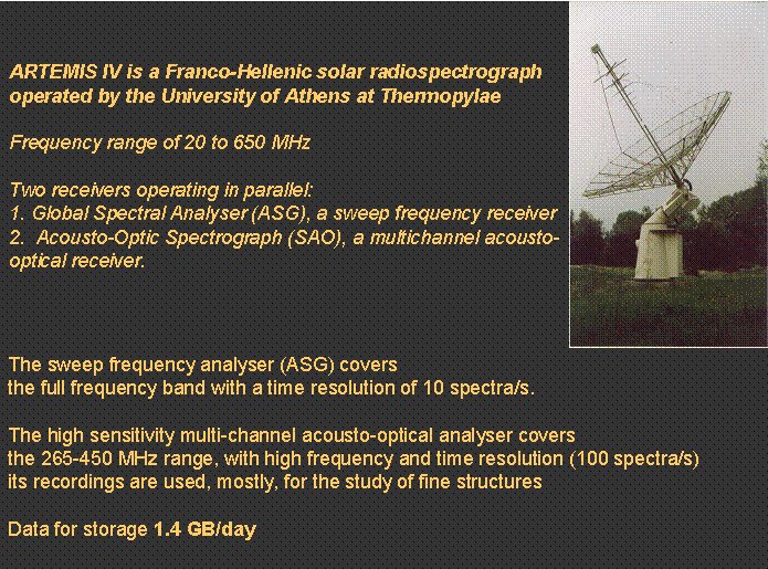
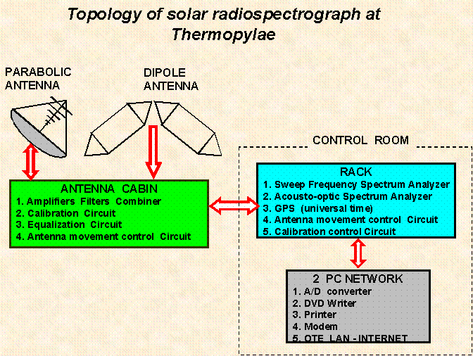
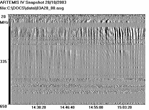
The Artemis IV solar radiospectrograph at Thermopylae is a complete system that
receives and records the dynamic spectrum of solar radio bursts on a daily
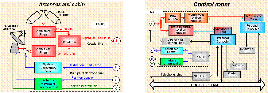
basis figure1 .figure5. It consists of:
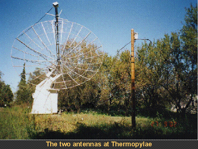
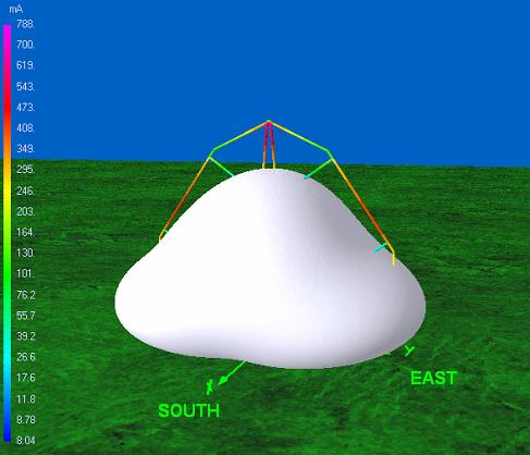
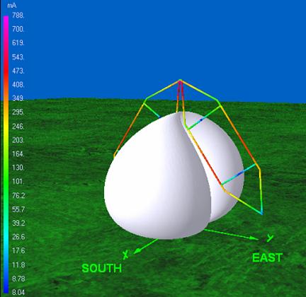
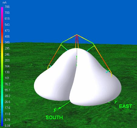
· Two antennas figure4 (one stationary for
the 20-110MHz band figure3 and one pointing to the
sun for the 110-650MHz figure2 ) and their cabin where
there are amplifiers, filters, a combiner, the calibration circuit and the
antenna movement circuit figure5 figure6
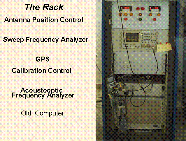
· The control room where there is a rack with two spectrum analyzers one
sweep for the whole range 20-650MHz and one acousto-optic for the range
270-450MHz, a GPS for receiving Universal Time, the control of the calibration
and the antenna movement circuits figure7. There
are also two PCs equipped with A/D cards, network cards, modem, and DVD Writer figure8
The distance between the antennas
with their cabin and the control room is 70m. An underground low loss 50 Ω coaxial line transmits the radio signal from the
antenna cabin to the control room and a multi pair line transmits the various
control and indication signals between the control room and the cabin figure6.
The output signal from every
spectrum analyzer is driven to two PCs where it is digitized, real time mapped
on the screen, storaged on the hard disk and at the
end of the daily observation the data are transferred to a DVD.figure8
The two PCs are connected via
Ethernet and via the OTE Lan they are connected to
the Internet. We can also control the whole operation via the telephone modem.
Later we study the data and
conclusions are derived for the solar events at the corona region figure10 figure11
The antennas
and their cabin
The solar radiospectrograph
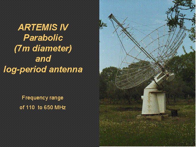
has a parabolic and a dipole antenna.
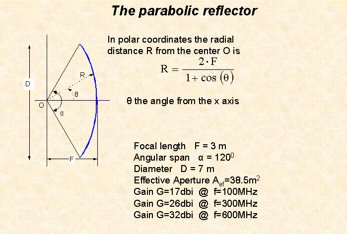
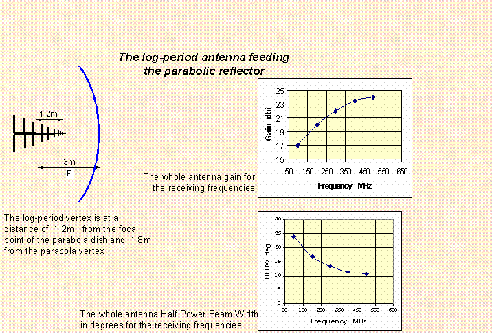
A. The parabolic antenna has a diameter of 7m, an angular span 1200,
focal length 3m and its reflective surface is made from a metal grid.figure12 On its axis, there two
identical log period antennas perpendicular each other’s for the 100-1000MHz
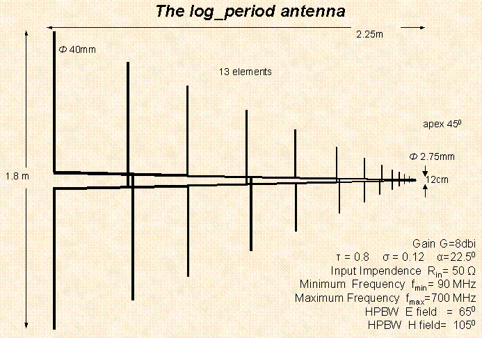
region. Each antenna has a length of 2.25m, apex angle 450 and
consists of 13 dipoles. figure13
At the present we use only the one log-period and therefore we receive only the
projection of the solar radio burst electric field on the antenna dipoles. This
combination gives a mean gain of 21db, a mean half power beamwidth
of 60 and 50Ω input
resistance.figure14 In future
we can use the two antennas to increase the sensitivity or to measure
polarization characteristics. The antenna has a typical equatorial mounting. It
can be rotated around two axes using motors and tracks the sun in declination
and hour angle.figure2 After
sunset the antenna moves automatically to the east. The antenna was designed in
France and constructed by the Greek company PYRKAL.
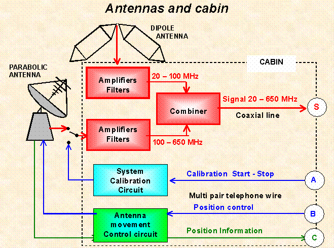
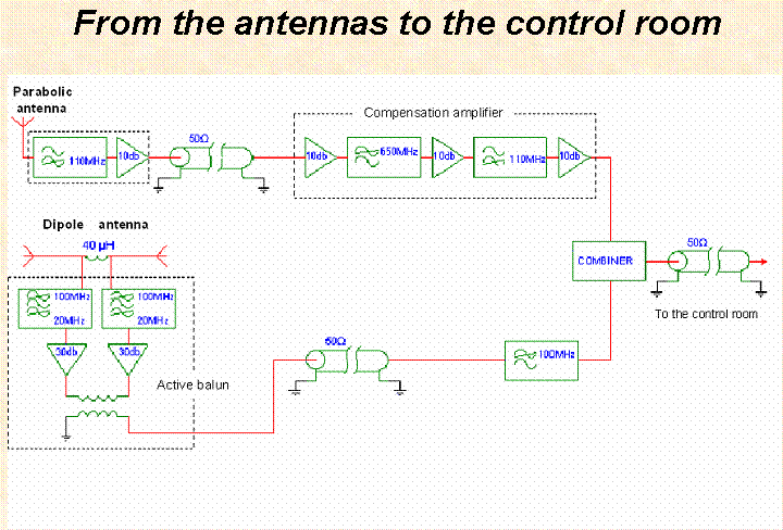
After collection the signal goes to
a 110 MHz high pass filter to reject strong FM radio broadcasting and a
pre-amplifier (10db gain and 3db noise figure) which are on the antenna.
Follows a compensation amplifier for the long transmission line. It is a
three-stage amplifier (30db total gain) with a low pass 650MHz and a high pass
110 MHz filter between them.figure15
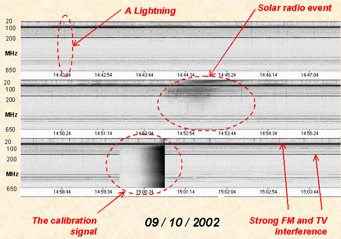
Every morning the system is
self-calibrated. The antenna is disconnected from the system and a white noise
generator (constant T=104 K) is connected. After this the noise
level is increased from 102 to 108
K linearly with time. The whole process lasts about 1 min and the signal is storaged. So we know the whole system behavior figure10
In the cabin there is the antenna
movement control circuit. Every morning the antenna starts its motion from hour
angle –72.50. Its constant angular velocity is 150/houre (equal to the sun angular velocity) and at the end it
reaches at 72.50 hour angle. The declination angle that changes 230/3
months is manually controlled by the position control system or remotely
through the modem. We observe the antenna position at indicators on the rack
and the sun position on the PC screen. The position control as the calibration
control is performed through the PC serial port. figure7
figure9
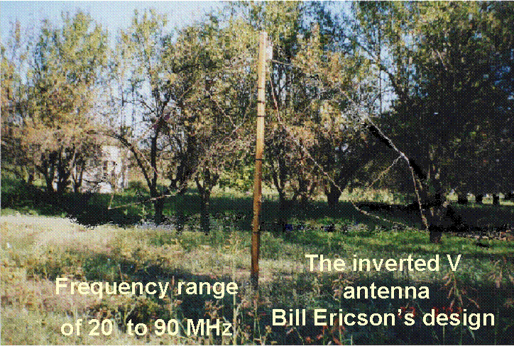
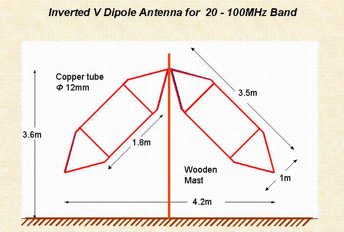
B. The dipole antenna is a very fat inverted V dipole on the east-west plane.
Every leg has an overall length 3.5 m and a width of 1m. It is constructed by
15mm diameter copper tube. The two legs form a 900 corner and its
apex is 3.6m above ground.figure16 figure3
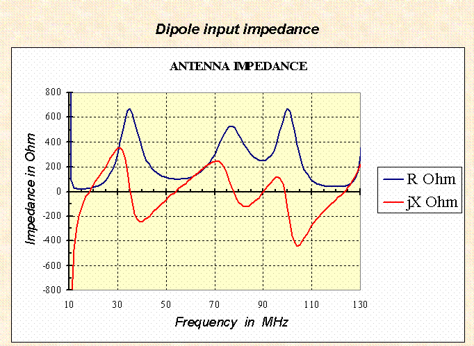
It has a resonance frequency at about 45 MHz with a
very large bandwidth because it is very fat. figure17 The floating over ground input impedance is
about 200Ω for
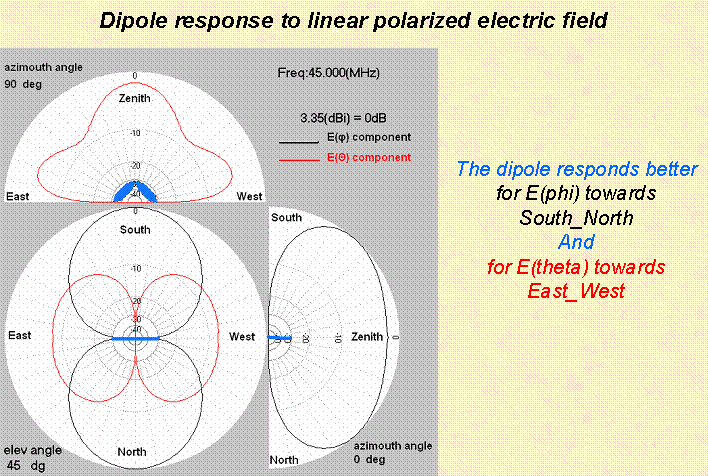
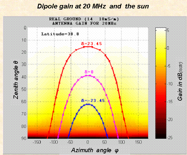
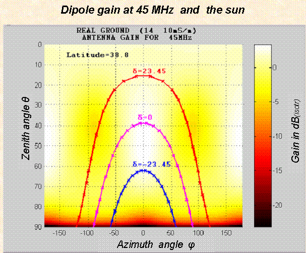
frequencies from 20 to 100MHz. The antenna receives vertically polarized
signals from low angles over the horizon from east-west and horizontally
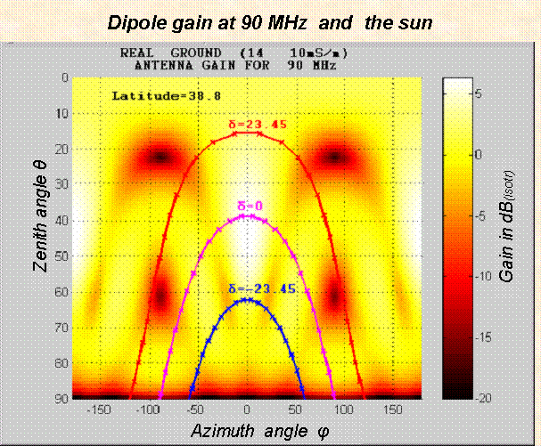
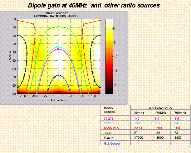
polarized signals from high angles over the horizon from south-north.figure18 figure34 figure35 figure36 So we can receive the sun signals during all the day and a
lot of interfering signals. figure19 figure20 figure21 figure22 figure29 figure30
After collection the signal goes
through a floating high pass and a low pass chebyshev
ninth order filter (fH=20 MHz and fL=90MHz) to avoid interference from strong
short wave and FM broadcasting. Follows an active balun
–amplifier constructed by two hybrid broadband
amplifiers ( Motorola CA 2832.) whose output are combined with the
primary coil of an rf transformer. The secondary coil
drives a coaxial 50 Ω
transmission line. The overall amplification is about 30db figure15
Follows a low pass filter (fL=90MHz) in order to protect the other antenna
signal from possible harmonics generated by the active balun.
A combiner combines the signals from the two antennas and drives them to the
control room through the long transmission line .
The control
room
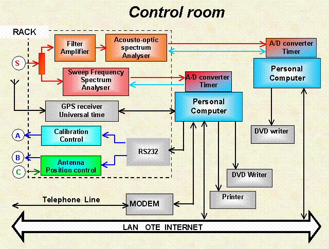
A splitter divides the signal from
the transmission line in two ways.figure8
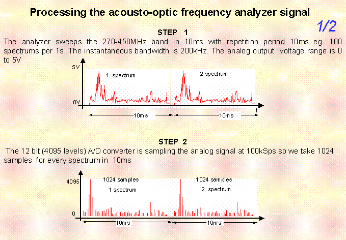
First way. It includes a classical sweep frequency analyzer (Analyseur de Spectre Global or
ASG) which covers the whole range from 20 to 650MHz at 10 sweeps/sec with
instantaneous bandwidth 1MHz and logarithmic amplification with dynamic range
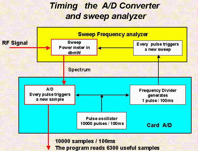
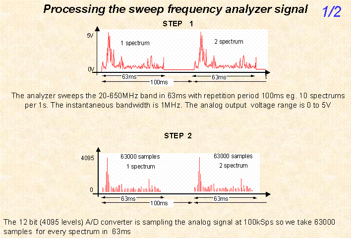
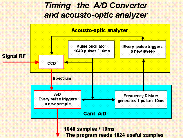
of 70 db. A pulse from a timer on the ADC card triggers every sweep. figure23
The analog output from the ASG drives an ADC card (Kethley 3100) on a PC. A timer on the card generates a
pulse every 100msec (frequency 10 Hz) which triggers the ASG to begin a new
frequency sweep. In 63msec the ASG sweeps the range from 20 to 650 MHz with
instantaneous bandwidth 1MHz and the ADC takes 6300 samples with a resolution
of 12bit. figure24 The samples
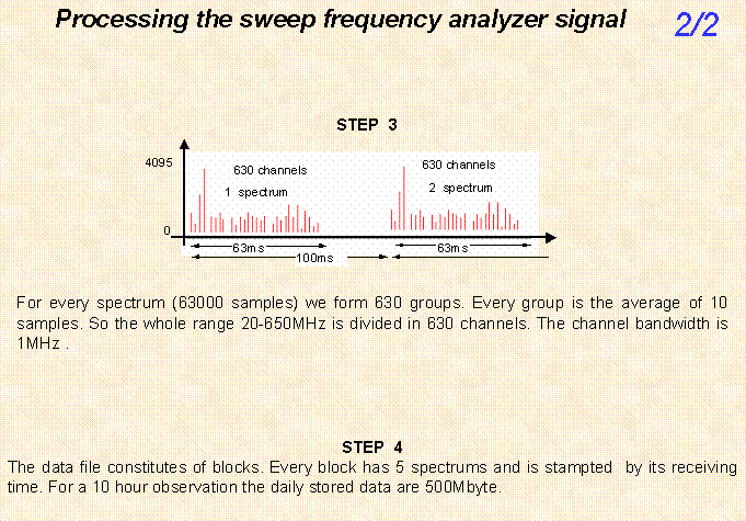
are averaged by ten so we have divide the whole spectrum to 630 channels with
resolution bandwidth 1MHz. If in a channel (10 samples) some measurements
correspond to the constant frequencies of strong FM radio or TV broadcasting we
average by the number of the useful ‘un-infected’ measurements. If in a channel
all the measurements are ‘infected’ we replace its intensity by the average of
the two adjacent channels. This arrangement leads to a high signal to noise
ratio.figure25 Every 5 sweeps
the measurements are transferred to the hard disk with a universal time stamp.
The 5 spectrums with the time stamp constitute a data block. Simultaneously we
see the dynamic spectrum on the PC screen. At the end of the day or later we
can take the daily activity and storage it on a DVD. The daily data are about
0.5Gbyte.
Every morning, before taking
measurements, this PC receives the Universal Time from a GPS through one serial
port to correct its clock. Also this PC controls the starting of the parabolic
antenna movement (when the hour angle of the sun is –72.50) and the
self-calibration procedure through the other serial port.
This PC is equipped with a
telephone line modem so whenever we can watch, receive the daily activity, and
if it is necessary we can control manually the system. Also there is an ethernet connection with the other PC
Second way: It includes a pass band filter 270-450 MHz, RF
amplifier, and finally an acousto-optic frequency analyzer (Spectrograph
Acousto-Optic, SAO) for the above frequency range with low dynamic linear range
(20db), very good frequency resolution at 176kHz and very fast frame rate at
100Hz. The SAO output drives an ADC card at the second PC. figure8
The SAO output comes from the
discharge of a linear CCD with 1024 pixel so that every pixel corresponds to a
different frequency. A correct sampling demands synchronization between the SAO
and the ADC card. For this reason the SAO pulses that trigger the pixel output
(1024 pulses in 10msec) drive and the ADC sampling.figure26 Also these pulses drive a frequency divider (on
the ADC card) which gives a pulse every 10msec. Every one of these pulses
triggers a new frame of the SAO.
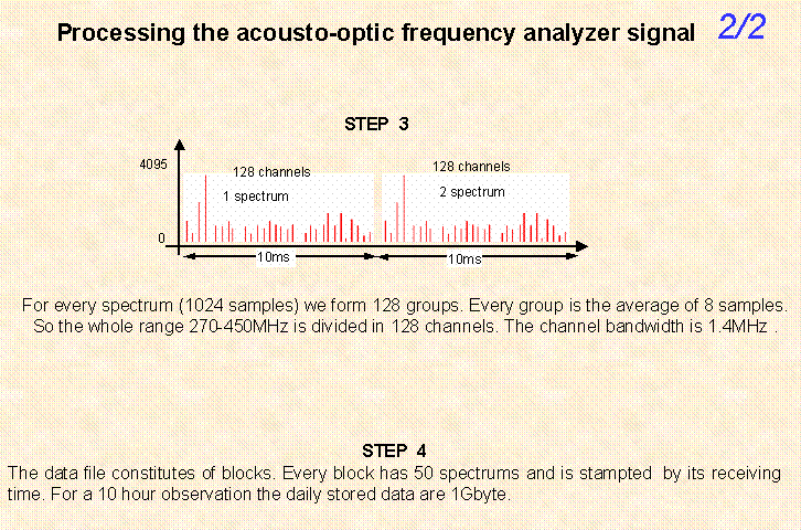
Finally every 10msec the SAO sweep
the range from 270 to 450 MHz with instantaneous bandwidth 176kHz
and the ADC takes 1024 samples with a resolution of 12bit. The samples are
averaged by eight, so we have divide the whole spectrum to 128 channels with
resolution bandwidth 1.4MHz.figure27
This arrangement leads to a high signal to noise ratio. Every 50 sweeps the
measurements are transferred to the hard disk with a universal time stamp. The
50 spectrums with the time stamp constitute a data block. Simultaneously we see
the dynamic spectrum on the PC screen.figure28
At the end of the day or later we can take the daily activity and storage it on
a DVD. The daily data are about 1Gbyte. The Universal Time is received every
morning from the other PC through the Ethernet.
Conclusions
and perspectives
This instrument has a very high
time and frequency resolution from decimeter to decameter wavelengths with a
very good signal to noise ratio, so we can distinguish fine structure at solar
radiobursts.figure31 figure32 figure33Future perspectives are the use of the old and
construction of new antenna to make polarimetric measurements
and extension of the SAO frequency range.
References
1.
C.Caroubalos, D. Maroulis, N. Patavalis, J.-l. Bougeret, G. Doumas, C. Perche, C. Alissandrakis, A. Hillaris, X.
Moussas, P. Preka-Papadema, A. Kontogeorgos, P. Tsitsipis, G. Kanelakis: 2001 ”The new multichannel radiospectrograph
ARTEMIS-IV/HECATE of the University of Athens” Experimental
Astronomy 11, 23-32
2.
William C. Erickson Professor at Utas University of Australia.private
communication.
3.
http://www.lofar.org
4.
Kethley KPCI 3100 ADC
manual.